• Data Structure
  • Hash Tabls
    • Direct-address Tables
    • Hash Tables
    • Hash Functions
      • The division method
      • The multiplication method
    • Open addressing
  • Binary Search Trees
    • Ordered Elements
    • Insertion
    • Deletion
  • Augmenting Data Structures
    • Order Statistic Tree
    • How to augment a datastructure

Data Structure

Hash Tabls

Direct-address Tables

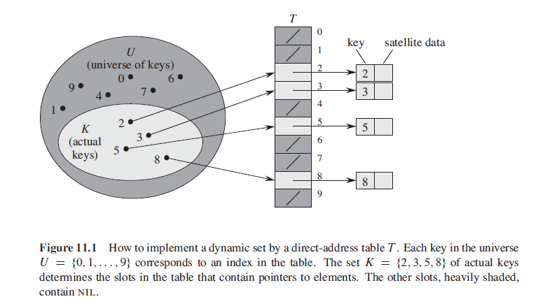
To represent the dynamic set, we use an array, or direct-address table, denoted by T[o,…,m-1], in which each position, or slot, corresponds to a key in the universe U. So it’s actually one-on-one and each slot can only contain one element.

Hash Tables

With hashing, this element is stored in slot h(k), that is, we use a hash function h to compute the slot from the key k. Here, h maps the universe U of keys into the slots of a hash table T(0,…,m-1) where the size m of the hash table is typically much less than |U|.

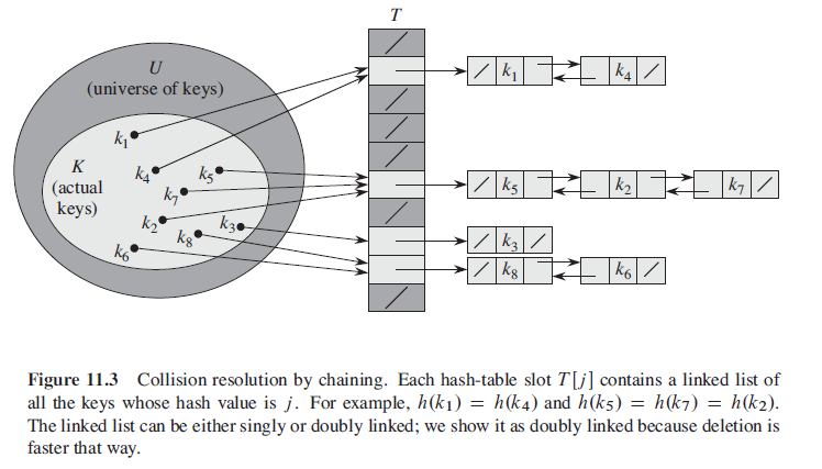
slot factor α = n/m which means expected length E[n_h(k)] = α.

Theorem In a hash table in which collisions are resolved by chaining, a successful search takes average-case time O(1+α) under the assumption of simple uniform hashing.

Hash Functions

It’s important to write a functionally good hash function, but what makes a good hash function?

A good hash function satisfies (approximately) the assumption of simple uniform hashing: each key is equally likely to hash to any of the m slots, independently of where any other key has hashed to.

The division method

h(k) = k mod m But choosing m = 2^p - 1 when k is a character string interpreted in radix 2p may be a poor choice, because permuting the characters of k does not change its hash value. An optimal choice is that we could choose m D 701 because it is a prime near 2000=3 but not near any power of 2.

The multiplication method

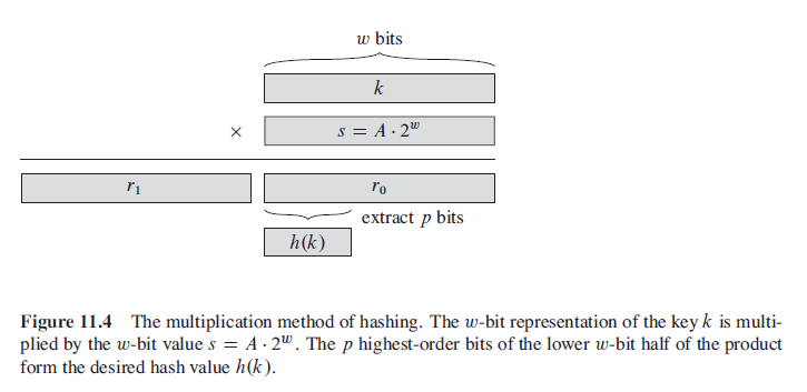
The multiplication method for creating hash functions operates in two steps. First, we multiply the key k by a constant A in the range 0 < A < 1 and extract the fractional part of kA. Then, we multiply this value by m and take the floor of the result. In short, the hash function is

h(k) = m(kA mod 1)

Open addressing

Unlike the hashtable with linked list, in open addressing, all elements occupy the hash table itself. That is, each table entry contains either an element of the dynamic set or NIL.

The main advantage of open addressing is to avoid use of pointer all together so we can have more memory.

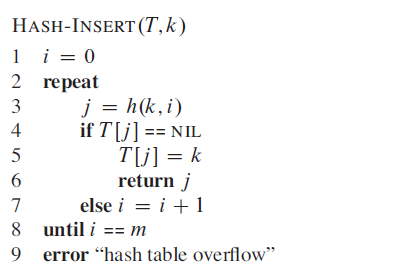
open addressing still use hash function, but when the index of h(x) is occupid, we do not create linked list for collision, but instead we move to the next index to see whether it’s occupid until we meet a NIL and put the data into it.

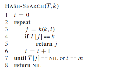
Same thing with searching, we simply start searching from the index of h(x) until we meet the result(success) or the NIL/end of the array(fail).

Binary Search Trees

A binary search tree is organized, as the name suggests, in a binary tree. In addition to a key and satellite data, each node contains attributes left, right, and p that point to the nodes corresponding to its left child, its right child, and its parent, respectively.

Let x be a node in a binary search tree. If y is a node in the left subtree of x, then y.key ≤ x.key. If y is a node in the right subtree of x, then y.key ≥ x.key.

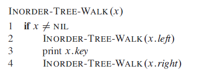
Ordered Elements

Since BST has already been sorted, we can easily print out all the elements in the BST in order.

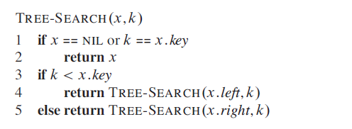
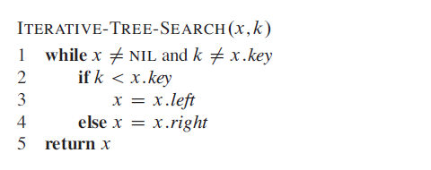
Also searching the BST is easy, there are two ways to do so, iteration and recursion.

Insertion

Insertion can take O(lgn) time, you just need to search down until meet the proper place and insert the new node.

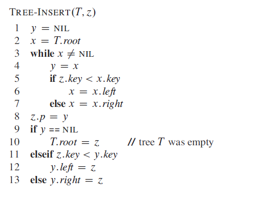
first using x and y to iterate down to find the “THE ONE” for our new node z. And when the loop ends, x is null and y is its parent. Finally we set z as y’s child consider their relative value.

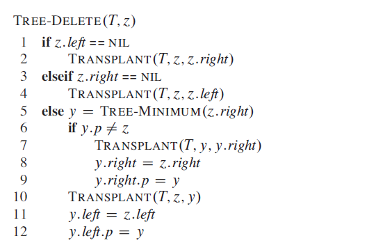
Deletion

Here comes the most complicated problem, deletion, which you should consider several cases.

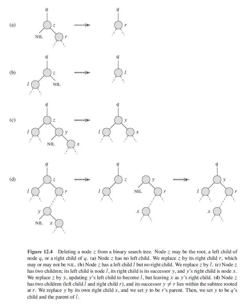
1. CASE 1: If z has no children, then we simply remove it by modifying its parent to replace z with NIL as its child.
2. CASE 2: If z has just one child, then we elevate that child to take z’s position in the tree by modifying z’s parent to replace z by z’s child.
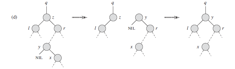
3. CASE 3: If z has two children, then we find z’s successor y—which must be in z’s right subtree—and have y take z’s position in the tree. The rest of z’s original right subtree becomes y’s new right subtree, and z’s left subtree becomes y’s new left subtree. This case is the tricky one because, as we shall see, it matters whether y is z’s right child.

The while process seems quite complicated, especially when with two chldren, but it’s actually simple.

For CASE 1, there’s nothing to say, just delete it.

For CASE 2, you just replace the deleted node with its child.

For CASE 3, first we find the minimum number at z.right, which we call it y, is the closest number with z.value, and relace z with y. Then y.right = z.right which put the original right subtree to y.right. Since y is the minimum number, it doesn’t have left child, and we put the y.right to y.parent.left where y originally lies.

specifically, this process:

Augmenting Data Structures

Order Statistic Tree

In practice, we do not usually use the texybook algorithm, instead we will nees to improve, or augment some structure. First we learn an augmented red-black tree.

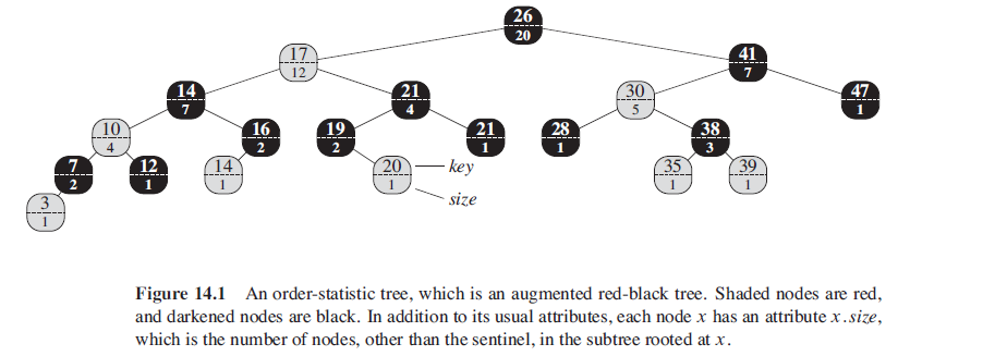
It’s based on red-black tree and we add a size attribute into the node. This attribute contains the number of (internal) nodes in the subtree rooted at x (including x itself), that is, the size of the subtree. And we have:

x.size = x.left.size + x.right.size + 1

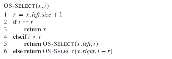
The procedure OS-SELECT(x,i) returns a pointer to the node containing the i th smallest key in the subtree rooted at x. To find the node with the i th smallest key in an order-statistic tree T , we call OS-SELECT(t.root,i).

Given a pointer to a node x in an order-statistic tree T , the procedure OS-RANK returns the position of x in the linear order determined by an inorder tree walk of T .

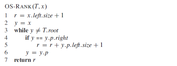
It add all the left subtree prior to node x.

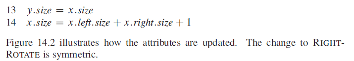
In the mean time, we can tell that other operation should be slightly modified. For example the LEFT-ROTATE should also change node.size.

How to augment a datastructure

There are few steps we need to follow:

1. Choose an underlying data structure.
2. Determine additional information to maintain in the underlying data structure.
3. Verify that we can maintain the additional information for the basic modifying operations on the underlying data structure.
4. Develop new operations.

We followed these steps design our order-statistic trees.

1. Step 1 we chose red-black trees as the underlying data structure. A clue to the suitability of red-black trees comes from their efficient support of other dynamicset operations on a total order, such as MINIMUM, MAXIMUM, SUCCESSOR, and PREDECESSOR.

2. Step 2, we added the size attribute, in which each node x stores the size of the subtree rooted at x. Generally, the additional information makes operations more efficient. For example, we could have implemented OS-SELECT and OS-RANK using just the keys stored in the tree, but they would not have run in O(lg n) time. Sometimes, the additional information is pointer information rather than data.

3. Step 3, we ensured that insertion and deletion could maintain the size attributes while still running in O(lg n) time. Ideally, we should need to update only a few elements of the data structure in order to maintain the additional information. For example, if we simply stored in each node its rank in the tree, the OS-SELECT and OS-RANK procedures would run quickly, but inserting a new minimum element would cause a change to this information in every node of the tree. When we store subtree sizes instead, inserting a new element causes information to change in only O(lg n) nodes.

4. Step 4, we developed the operations OS-SELECT and OS-RANK. After all, the need for new operations is why we bother to augment a data structure in the first place. Occasionally, rather than developing new operations, we use the additional information to expedite existing ones.