• Advanced Design
  • Dynamic Programming
    • How to Design an Algorithm Using Dynamic Programming
      • Characterize the structure of an optimal solution
      • Recursively define the value of an optimal solution
      • Compute the value of an optimal solution
      • Construct an optimal solution from computed information
    • When Can We use Dynamic Programming
      • Optimal Substructure
        • Common Pattern
        • Independency
      • Overlapping Subproblems
      • Memoization
    • Longest Common Subsequence
      • Step 1: Characterizing a longest common subsequence
      • Step 2: A recursive solution
      • Step 3: Computing the length of an LCS
      • Step 4: Constructing an LCS
    • Problems
      • Planning an investment strategy
      • Inventory planning
      • Signing free-agent baseball players
  • Amortized Analysis
    • Aggregate analysis
    • The accounting method
    • The potential method

Advanced Design

Dynamic Programming

This chapter is quite hard yet useful. It seems the implementation is complicated but the main idea is all the same and simple which we do not calculate the same thing more than once. It’s often the case that we keep an array or a table to keep the value we already calculated and the next problem are gonna solve will depend on the previous answer that been stored in the array.

How to Design an Algorithm Using Dynamic Programming

we shall follow the four-step sequence:

1. Characterize the structure of an optimal solution.

2. Recursively define the value of an optimal solution.

3. Compute the value of an optimal solution.

4. Construct an optimal solution from computed information.

Talk is cheap, show me the example.

We will follow this four steps to solve the Matrix-chain multiplication problem.

Characterize the structure of an optimal solution

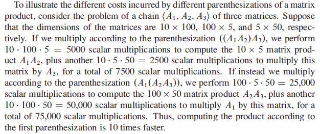
To compute the matrix multiplication, say A_ij and B_jk, we need ijk time units. So Matrix-chain multiplication varies with order of multiplication.

Now we use our optimal substructure to show that we can construct an optimal solution to the problem from optimal solutions to subproblems.

Recursively define the value of an optimal solution

Let m(i,j) be the minimum number of scalar multiplications needed to compute the matrix A_i…j; for the full problem, the lowestcost way to compute A_i…n would thus be m(1,n).

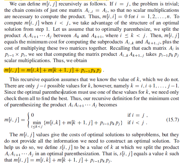
It’s almost the most important part to figure out the formula:

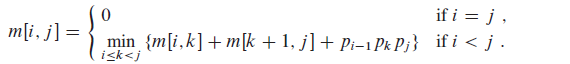
Only in this way can we preceed to wirthe the code for computing.

Compute the value of an optimal solution

Now we konw the formula, and the code is writing itself.

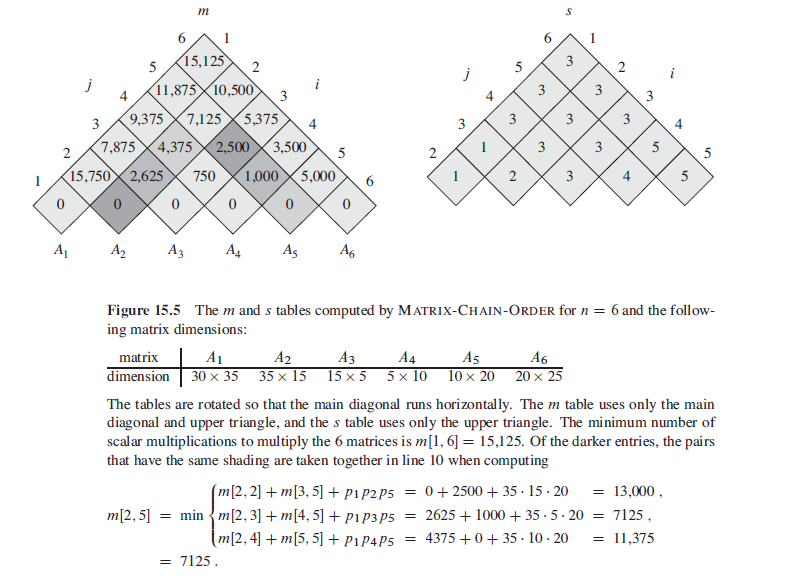
We will uses an auxiliary table m[1…n,1…n] for storing the m[i,j] costs and another auxiliary table s[1…n-121…n] that records which index of k achieved the optimal cost in computing m[i,j]. We shall use the table s to construct an optimal solution.

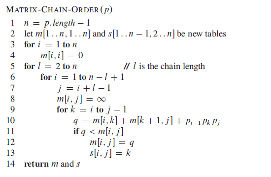
Then we can have a table keep the time units will be spent with different i and j.

Construct an optimal solution from computed information

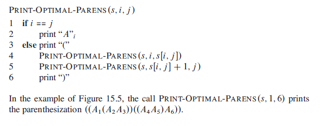
Finally, since we have table m and s, we can construct our solution:

When Can We use Dynamic Programming

It’s a great improvent if we implement dynamic programming, but when should we look for a dynamic-programming solution to a problem?

There are two key ingredients that an optimization problem must have in order for dynamic programming to apply:

• optimal substructure and
• overlapping subproblems.

Optimal Substructure

The first step in solving an optimization problem by dynamic programming is to characterize the structure of an optimal solution.

a problem exhibits optimal substructure if an optimal solution to the problem contains within it optimal solutions to subproblems.

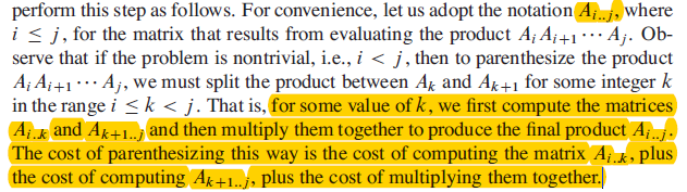
For example, we observed that an optimal parenthesization of A_iA_i+1……A_j that splits the product between A_k and A_k+1 contains within it optimal solutions to the problems of parenthesizing A_i……A_k and A_k+1……A_j .

Common Pattern

You will find yourself following a common pattern in discovering optimal substructure:

1. You show that a solution to the problem consists of making a choice, such as choosing an initial cut in a rod or choosing an index at which to split the matrix chain. Making this choice leaves one or more subproblems to be solved.
2. You suppose that for a given problem, you are given the choice that leads to an optimal solution. You do not concern yourself yet with how to determine this choice. You just assume that it has been given to you.
3. Given this choice, you determine which subproblems ensue and how to best characterize the resulting space of subproblems.
4. You show that the solutions to the subproblems used within an optimal solution to the problem must themselves be optimal by using a “cut-and-paste” technique. You do so by supposing that each of the subproblem solutions is not optimal and then deriving a contradiction. In particular, by “cutting out” the nonoptimal solution to each subproblem and “pasting in” the optimal one, you show that you can get a better solution to the original problem, thus contradicting your supposition that you already had an optimal solution. If an optimal solution gives rise to more than one subproblem, they are typically so similar that you can modify the cut-and-paste argument for one to apply to the others with little effort.

Independency

There are some cases we should not use dynamic programm.

Here’s an example.

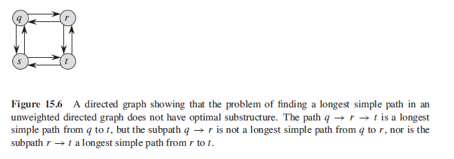
The reason why dynamic programming doesn’t work is that two subproblems are not independent. Independency mean that the solution to one subproblem does not affect the solution to another subproblem of the same problem.

For the example, we have the problem of finding a longest simple path from q to t with two subproblems: finding longest simple paths from q to r and from r to t . For the first of these subproblems, we choose the path q–>s–>t–>r, and so we have also used the vertices s and t . We can no longer use these vertices in the second subproblem, since the combination of the two solutions to subproblems would yield a path that is not simple. If we cannot use vertex t in the second problem, then we cannot solve it at all. Because we use vertices s and t in one subproblem solution, we cannot use them in the other subproblem solution. We must use at least one of them to solve the other subproblem. Thus, we say that these subproblems are not independent. Looked at another way, using resources in solving one subproblem (those resources being vertices) renders them unavailable for the other subproblem.

All above means that the subproblems do not share resources.

Overlapping Subproblems

The second ingredient that an optimization problem must have for dynamic programming to apply is that the space of subproblems must be “small” in the sense that a recursive algorithm for the problem solves the same subproblems over and over, rather than always generating new subproblems. Typically, the total number of distinct subproblems is a polynomial in the input size. When a recursive algorithm revisits the same problem repeatedly, we say that the optimization problem has overlapping subproblems.

In contrast, a problem for which a divide-andconquer approach is suitable usually generates brand-new problems at each step of the recursion. Dynamic-programming algorithms typically take advantage of overlapping subproblems by solving each subproblem once and then storing the solution in a table where it can be looked up when needed, using constant time per lookup.

Memoization

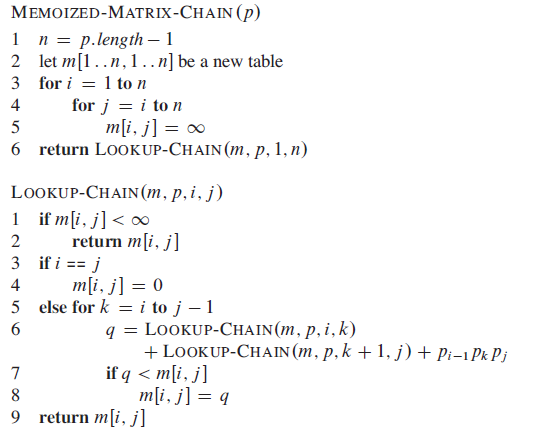
As we saw for the rod-cutting problem, there is an alternative approach to dynamic programming that often offers the efficiency of the bottom-up dynamicprogramming approach while maintaining a top-down strategy. The idea is to memoize the natural, but inefficient, recursive algorithm. As in the bottom-up approach, we maintain a table with subproblem solutions, but the control structure for filling in the table is more like the recursive algorithm.

A memoized recursive algorithm maintains an entry in a table for the solution to each subproblem. Each table entry initially contains a special value to indicate that the entry has yet to be filled in. When the subproblem is first encountered as the recursive algorithm unfolds, its solution is computed and then stored in the table. Each subsequent time that we encounter this subproblem, we simply look up the value stored in the table and return it.

Top-Down(Top elements first, recursive)

Bottom-up(Bottom elements first, iteration)

The main advantage of memouzation is that it only calculate the data we need, so for some problem that does not require all the data, it can save lots of time.

In general practice, if all subproblems must be solved at least once, a bottom-up dynamic-programming algorithm usually outperforms the corresponding top-down memoized algorithm by a constant factor, because the bottom-up algorithm has no overhead for recursion and less overhead for maintaining the table. Moreover,for some problems we can exploit the regular pattern of table accesses in the dynamicprogramming algorithm to reduce time or space requirements even further. Alternatively, if some subproblems in the subproblem space need not be solved at all, the memoized solution has the advantage of solving only those subproblems that are definitely required.

Longest Common Subsequence

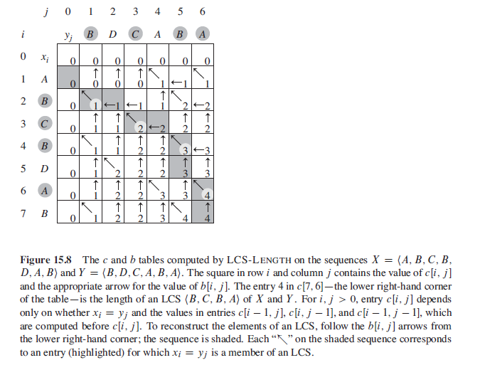
Given two sequences, X=<A,B,C,B,D,A,B>, Y=<B,D,C,A,B,A>, and <B,C,B,A>,<B,C,A,B> are both their Longest Common Subsequence or LCS.

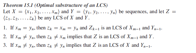
Step 1: Characterizing a longest common subsequence

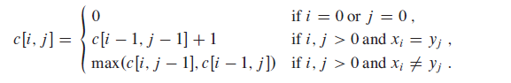
Step 2: A recursive solution

Let us define c[i,j] to be the length of an LCS of the sequences X_i and Y_j.

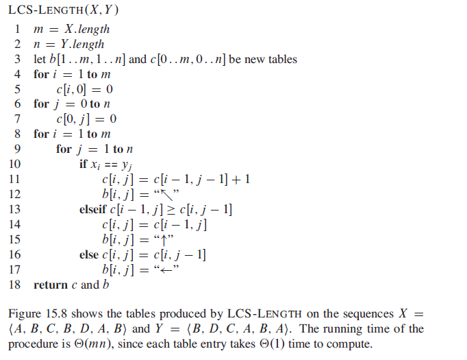
Step 3: Computing the length of an LCS

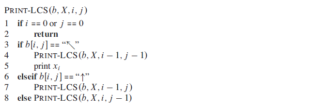
Step 4: Constructing an LCS

Problems

These problems might be helpful for better understanding

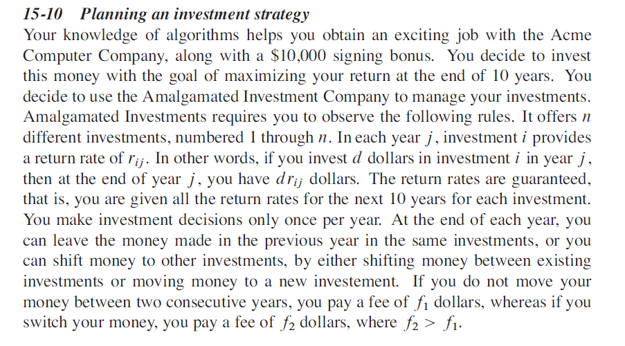
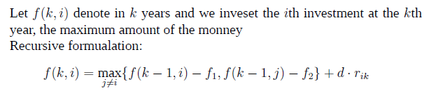
Planning an investment strategy

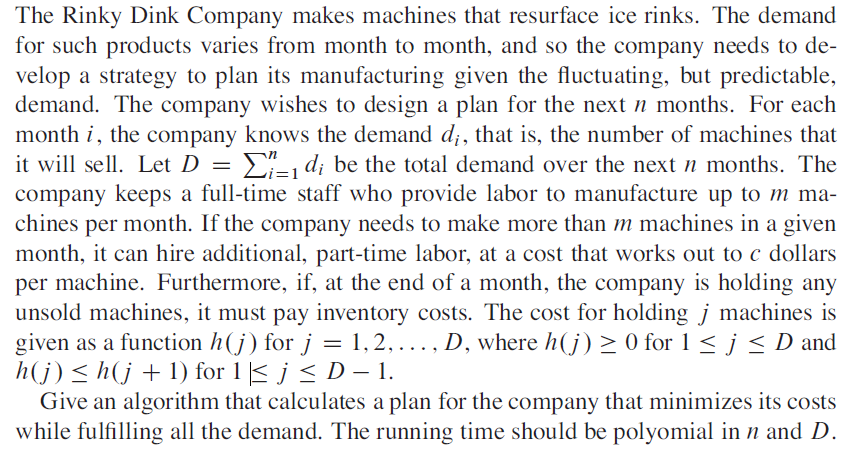
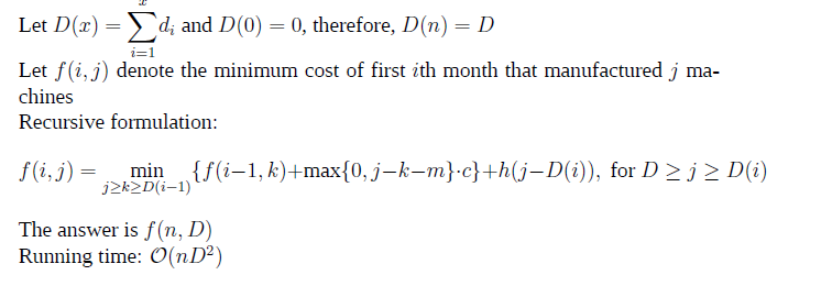
Inventory planning

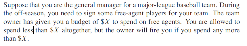
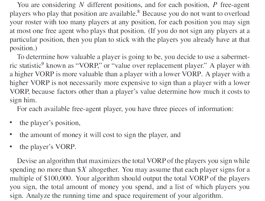
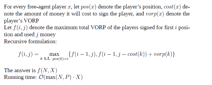
Signing free-agent baseball players

Amortized Analysis

It’s true that we can get worst running time by assuming the worst case, but often the case we don’t meet the worst situation. So we need to use Amortized Analysis to compute the average running time.

Amortized analysis differs from average-case analysis in that probability is not involved; an amortized analysis guarantees the average performance of each operation in the worst case.

Aggregate analysis

In aggregate analysis, we show that for all n, a sequence of n operations takes worst-case time T(n) in total. In the worst case, the average cost, or amortized cost, per operation is therefore T(n)/n.

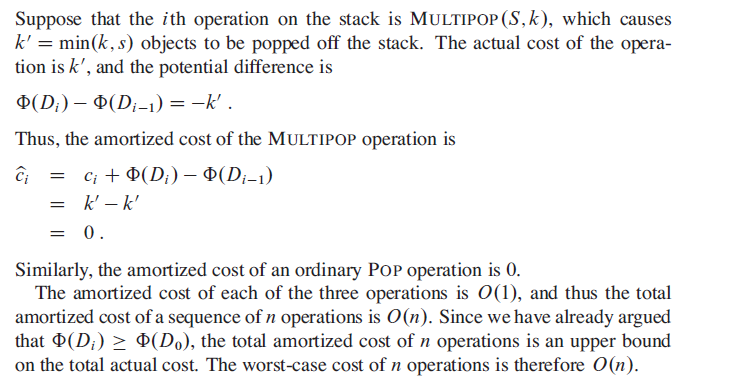
We define MULTIPOP(S,k) as pop k elements from Stack S which takes k units time.

Although a single MULTIPOP operation can be expensive, any sequence of n PUSH, POP, andMULTIPOP operations on an initially empty stack can cost at most O(n).Because We can pop each object from the stack at most once for each time we have pushed it onto the stack. Therefore, the number of times that POP can be called on a nonempty stack, including calls within MULTIPOP, is at most the number of PUSH operations, which is at most n.

In this example, therefore, all three stack operations have an amortized cost of O(1).

The accounting method

When an operation’s amortized cost exceeds its actual cost, we assign the difference to specific objects in the data structure as credit. Credit can help pay for later operations whose amortized cost is less than their actual cost. Thus, we can view the amortized cost of an operation as being split between its actual cost and credit that is either deposited or used up.

We assign the following amortized costs:

• PUSH 2
• POP 0
• MULTIPOP 0

Note that the amortized cost of MULTIPOP is a constant (0), whereas the actual cost is variable. Because we already pay for each pop action when they are pushed in.

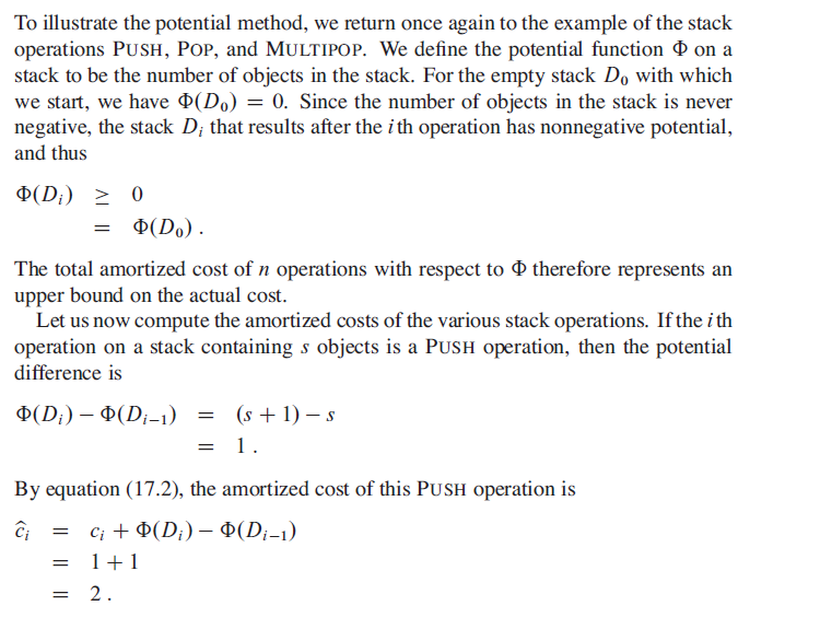
The potential method

the potential method of amortized analysis represents the prepaid work as “potential energy,” or just “potential,” which can be released to pay for future operations.

For each i = 1,2,3,…,n, we let c_i be the actual cost of the i th operation and D_i be the data structure that results after applying the i th operation to data structure D_i-1.